General pipeline usage

After composing a project directory with raw data, marker specification, and parameters, provide the entire directory to the pipeline via --in:

# Get the latest version of the pipeline
nextflow pull labsyspharm/mcmicro

# Run the pipeline on data
nextflow run labsyspharm/mcmicro --in path/to/my/project/

(Where path/to/my/project/ is replaced with your specific path.)

Input

At the minimum, the pipeline expects two inputs

1. markers.csv in the parent directory (containing metadata with markers)
2. Input images that are either
   • Raw image tiles placed in the raw/ subdirectory, or
   • Preregistered images placed in the registration/ subdirectory

Two other inputs are optional

1. (Optional) Precomputed Illumination profiles in the illumination/ subdirectory.
2. (Optional) A params.yml file specifying parameters. If not provided, MCMICRO will use default values.

An example input directory may look like

myproject/
├── markers.csv
├── params.yml
├── raw/
└── illumination/

Using pre-registered images

The canonical image processing workflow accepts as input raw, unstitched image tiles. If your tiles have already been stitched and registered across cycles, place the resulting OME-TIFF in the registration/ subdirectory instead. An example input directory may then look like

myproject/
├── markers.csv
├── params.yml
└── registration/
    └── myimage.ome.tif

The pipeline will then need to be configured to start with the segmentation step by adding the following workflow parameter to your params.yml:

workflow:
  start-at: segmentation

Markers

The file markers.csv must be in a comma-delimited format and contain a column titled marker_name that defines marker names of every channel:

Example markers file:

cycle,marker_name
1,DNA_1
1,AF488
1,AF555
1,AF647
2,DNA_2
2,A488_background
2,A555_background
2,A647_background
3,DNA_3
3,FDX1
3,CD357
3,CD1D

All other columns are optional but can be used to specify additional metadata (e.g., known mapping to cell types) to be used by individual modules.

Raw images

The exemplar raw/ files are in the open standard OME-TIFF format, but in practice your input files will be in whatever format your microscope produces. The pipeline supports all Bio-Formats-compatible image formats, but additional parameters may be required.

(Optional) Illumination corrected images

Pre-computed flat-field and dark-field illumination profiles can be placed in the illumination/ directory. If no pre-computed profiles are available, MCMICRO can compute these using BaSiC. This step is not executed by default, because proper illumination correction requires careful curation and visual inspection of the profiles produced by computational tools. After familiarizing yourself with the general concepts, the profiles can be computed by specifying a different starting point.

(Optional) Parameter file

The parameter file must be named params.yml and placed in the project directory, alongside markers.csv. Parameter values must be specified using standard YAML format. Please see the detailed parameter descriptions for more information.

Back to top

Output

Stitching and registration

ASHLAR is the default first step of the pipeline. ASHLAR will aggregate individual image tiles from raw/ along with the corresponding illumination profiles to produce a stitched and registered mosaic image.

This mosaic image will be published to the registration/ subdirectory:

exemplar-001
├── markers.csv
├── raw/
├── illumination/
└── registration/
    └── exemplar-001.ome.tif

The output filename will be generated based on the name of the project directory.

(Optional) TMA dearray

When working with Tissue Microarrays (TMA), Coreograph is used for TMA dearraying. The registration/ folder will contain an image of the entire TMA. Turn on the tma setting in workflow parameters to have MCMICRO identify and isolate individual cores.

Each core will be written out into a standalone file in the dearray/ subdirectory along with the mask specifying where in the original image the core appeared:

exemplar-002
├── ...
├── registration/
│   └── exemplar-002.ome.tiff
└── dearray/
    ├── 1.tif
    ├── 2.tif
    ├── 3.tif
    ├── 4.tif
    └── masks/
        ├── 1_mask.tif
        ├── 2_mask.tif
        ├── 3_mask.tif
        └── 4_mask.tif

All cores will then be processed in parallel by all subsequent steps.

Segmentation

Cell segmentation is carried out in two steps. First, the pipeline generates probability maps that annotate each pixel with the probability that it belongs to a given subcellular component (nucleus, cytoplasm, cell boundary) using UnMICST (default) or Ilastik. The second step applies standard watershed segmentation to produce the final cell/nucleus/cytoplasm/etc. masks using S3segmenter.

The two steps will appear in probability-maps/ and segmentation directories, respectively. When there are multiple modules for a given pipeline step, their results will be subdivided into additional subdirectories:

exemplar-001
├── ...
├── probability-maps/
│   ├── ilastik/
│   │   └── exemplar-001_Probabilities.tif
│   └── unmicst/
│       └── exemplar-001_Probabilities_0.tif
└── segmentation/
    ├── ilastik-exemplar-001/
    │   ├── cell.ome.tif
    │   └── nuclei.ome.tif
    └── unmicst-exemplar-001/
        ├── cell.ome.tif
        └── nuclei.ome.tif

Quantification

The final step, MCQuant, combines information in segmentation masks, the original stitched image and markers.csv to produce Spatial Feature Tables that summarize the expression of every marker on a per-cell basis, alongside additional morphological features (cell shape, size, etc.).

Spatial Feature Tables will be published to the quantification/ directory:

exemplar-001
├── ...
├── segmentation/
└── quantification/
    ├── ilastik-exemplar-001_cell.csv
    └── unmicst-exemplar-001_cell.csv

There is a direct correspondence between the .csv filenames and the filenames of segmentation masks. For example, quantification/unmicst-exemplar-001_cell.csv quantifies segmentation/unmicst-exemplar-001/cell.ome.tif.

Each .csv file will contain the following columns:

• CellID - cell index that is extracted from the segmentation mask
• All columns with names matching those in markers.csv - average intensity of that channel in the cell/nuclei area
• All other columns will contain morphological features.

Quality control

Additional information during pipeline execution will be written to the qc/ directory, by both individual modules and the pipeline itself.

exemplar-002
├── ...
└── qc
    ├── params.yml
    ├── provenance/
    │   ├── probmaps:ilastik (1).log
    │   ├── probmaps:ilastik (1).sh
    │   ├── probmaps:unmicst (1).log
    │   ├── probmaps:unmicst (1).sh
    │   ├── quantification (1).log
    │   ├── quantification (1).sh
    │   └── ...
    ├── coreo/
    ├── s3seg/
    └── unmicst/

While the exact content of the qc/ directory will depend on which modules were executed, two sources of information can always be found there:

1. The file params.yml will contain the full record of module versions and all parameters used to run the pipeline. This allows for full reproducibility of future runs.
2. The provenance/ subdirectory will contain exact commands (.sh) executed by individual modules, as well the output (.log) of these commands.

* You should retain params.yml and provenance/ because these files enable full reproducibility of a pipeline run. The other QC files can be safely deleted once the quality of the outputs has been verified and no more parameter tuning is expected.

The remaining directories will contain QC files specific to individual modules:

1. When working with TMAs, coreo/ will contain TMA_MAP.tif, a mask showing where in the original TMA image the segmented cores reside.
2. If UnMicst was used to generate probability maps, unmicst/ will contain thumbnail previews, allowing for a quick assessment of their quality.
3. After segmentation, two-channel tif files containing DAPI and nuclei/cell/cytoplasm outlines will reside in s3seg/, allowing for a visual inspection of segmentation quality.

Back to top

Directory Structure

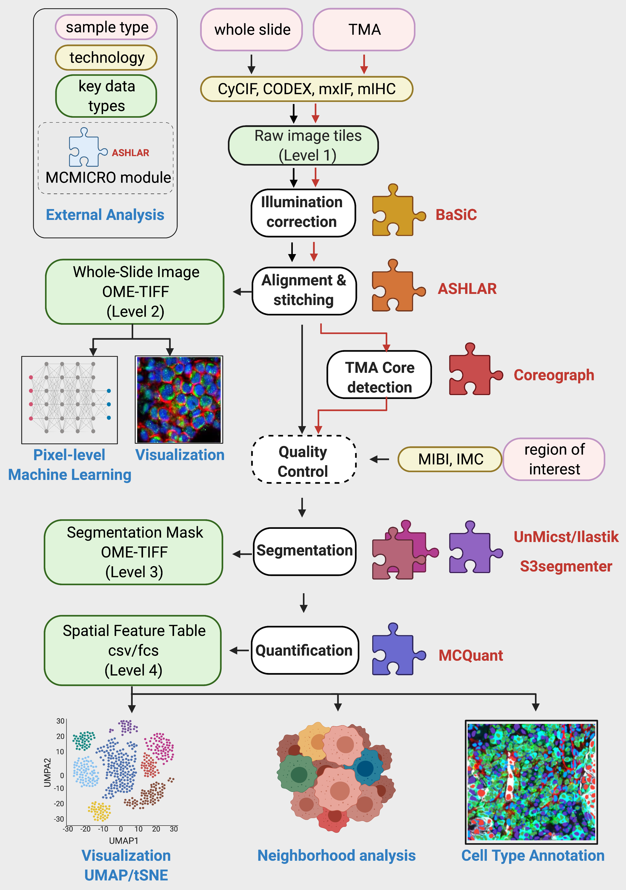
Upon the full successful completion of a pipeline run, the directory structure will follow Fig. 1A in the MCMICRO manuscript:

Note: This directory should correspond directly to the Nextflow workflow. For the Galaxy workflow, the intermediaries and output files should be identical, but the organization of the files within directories and the filenames will be different.

Schematic	Directory Structure
	exemplar-002 ├── markers.csv ├── raw/ ├── illumination/ ├── registration/ ├── dearray/ ├── probability-maps/ ├── segmentation/ ├── quantification/ └── qc/

The name of the parent directory (e.g., exemplar-002) is assumed by the pipeline to be the sample name.

Visual inspection of quality control (qc/) files is recommended after completing the run. Depending on the modules used, directories coreo/, unmicst/ and s3seg/ may contain .tif images for inspection.

By default Nextflow writes intermediate files to a work/ directory inside whatever location you initiate a pipeline run from. You can change that by specifying a different -w parameter.

Back to top