MCMICRO tutorial

Here we show an example of how to execute MCMICRO on two exemplar datasets using the command line (Nextflow) interface on a local computer.

Note: Nextflow is compatible with Linux or Mac (through the terminal), but Windows users will need to set up a Windows Subsystem for Linux or use the Galaxy workflow.

If you are not running MCMICRO on your local computer, please head to Platforms for platform-specific instructions.

Following this tutorial can verify that MCMICRO is correctly installed and running on your computer by demonstrating the expected inputs and outputs for the exemplar datasets.

Step 0: Be sure to install nextflow and Docker before proceeding through these steps.

Enter the commands nextflow run hello and docker run hello-world to verify that both Nexflow and Docker* are functional.

*If using a Windows environment, you may need to run Docker as Administrator.

*If using a MacOS environment, you may need to increase the amount of RAM allocated to Docker.

Step 1: Ensure you have the latest version of the pipeline

nextflow pull labsyspharm/mcmicro

Step 2: Download exemplar data.

Replace /my/path with where you want to store the files. (Use . for path to download files into the current directory.)

# Download exemplar-001
nextflow run labsyspharm/mcmicro/exemplar.nf --name exemplar-001 --path /my/path

# Download exemplar-002
nextflow run labsyspharm/mcmicro/exemplar.nf --name exemplar-002 --path /my/path

Both exemplar datasets have the directory structure of

exemplar-001 or exemplar-002
├── markers.csv
├── raw/
|   ├── exemplar-001-cycle-06.ome
|   ├── exemplar-001-cycle-07.ome
|   └── ...
|   
└── illumination/
    ├── ...
    ├── exemplar-001-cycle-06-dfp.tif
    ├── exemplar-001-cycle-06-ffp.tif
    ├── ...
    └── ...

NOTE: For this tutorial, we demonstrate running the pipeline with the input of raw images and illumination profiles (in illumination). To see a more comprehensive description of inputs for MCMICRO, please see the Input section under Inputs/Outputs.

By default, exemplar-001 contains cycles 6 through 8, while exemplar-002 contains all 10 cycles. Use nextflow run labsyspharm/mcmicro/exemplar.nf --help to learn how to download a different range of cycles for each exemplar.

Each cycle has one .ome.tif file in raw/ and two .tif files in illumination/. These images look like the following:

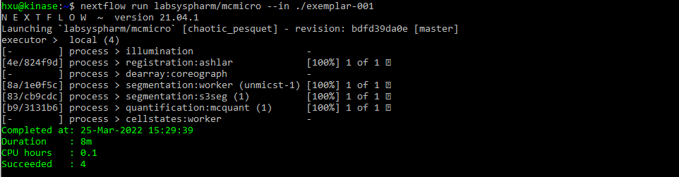
Step 3: Use --in to point the pipeline at the data.

In the commands below, /my/path should match what was used to download exemplar data with exemplar.nf command above (. can again be used to point to the current directory).

# Run the pipeline on exemplar data (starting from the registration step, by default)
nextflow run labsyspharm/mcmicro --in /my/path/exemplar-001

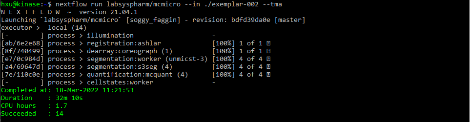
# params.yml in exemplar-002 will tell MCMICRO to treat data as a tissue microarray
nextflow run labsyspharm/mcmicro --in /my/path/exemplar-002

If your computer has an Apple M1 chip, you may need to specify ilastik for probability maps at this step. Read more on the FAQ page.

*On an average workstation, it takes approximately 5-10 minutes to process exemplar-001 from start to finish. Exemplar-002 is substantially larger, and takes 30-40 minutes on an average workstation.

After a successful run, the following text will be displayed for exemplar-001 and exemplar-002:

The pipeline will generate the following directory, depending on the modules used.

exemplar-001
├── markers.csv
├── raw/
├── illumination/
├── registration/
|  └── exemplar-001.ome
├── probability-maps/
|   └── unmicst/    
|       └── exemplar-001-pmap.tif
├── segmentation/
|   ├── cell.ome
|   └── nuclei.ome
├── quantification/
|   └── unmicst-exemplar-001_cell.csv
└── qc/
   ├── provenance/
   |   ├── quantification·mcquant(1).txt
   |   ├── quantification·mcquant(1).sh
   |   ├── reigstration·ashlar.txt
   |   ├── registration·ashlar.sh
   |   ├── segmentation·s3seg(1).txt
   |   ├── segmentation·s3seg(1).sh
   |   ├── segmentation·worker(unmicst-1).txt
   |   └── segmentation·workder(unmicst-1).sh
   ├── s3seg/
   |   └── unmicst-exemplar-001/
   |       ├── cellOutlines.ome
   |       └── nucleiOutlines.ome
   ├── unmicst/
   |   └── exemplar-001-Preview_1.tif
   └── params.yml

exemplar-002
├── markers.csv
├── raw/
├── illumination/
├── registration/
|   └── exemplar-002.ome
├── dearray/
|   ├── masks/
|   |   ├── 1_mask.tif
|   |   ├── 2_mask.tif
|   |   ├── 3_mask.tif
|   |   └── 4_mask.tif
|   ├── 1.tif
|   ├── 2.tif
|   ├── 3.tif
|   └── 4.tif
├── probability-maps/
|   └── unmicst/
|       ├── 1-pmap.tif
|       ├── 2_pmap.tif
|       ├── 3_pmap.tif
|       └── 4_pmap.tif   
├── segmentation/
|   ├── unmicst-1/
|   |   ├── cell.ome
|   |   └── nuclei.ome
|   ├── unmicst-2/
|   |   ├── cell.ome
|   |   └── nuclei.ome
|   ├── unmicst-3/
|   |   ├── cell.ome
|   |   └── nuclei.ome
|   └── unmicst-4/
|       ├── cell.ome
|       └── nuclei.ome
├── quantification/
|   ├── unmicst-1_cell.csv
|   ├── unmicst-2_cell.csv
|   ├── unmicst-3_cell.csv
|   └── unmicst-4_cell.csv
└── qc/
    ├──coreo/
    |  ├── centroidsY-X.txt
    |  └── TMA_MAP.tif
    ├── provenance/
    |   ├── dearraycoreograph(1).txt
    |   ├── dearraycoreograph(1).sh
    |   ├── quantification·mcquant(1).txt
    |   ├── quantification·mcquant(1).sh
    |   ├── ...
    |   ├── quantification·mcquant(4).txt
    |   ├── quantification·mcquant(4).sh 
    |   ├── reigstration·ashlar.txt
    |   ├── registration·ashlar.sh
    |   ├── segmentation·s3seg(1).txt
    |   ├── segmentation·s3seg(1).sh
    |   ├── ...
    |   ├── segmentation·s3seg(4).txt
    |   ├── segmentation·s3seg(4).sh 
    |   ├── segmentation·worker(unmicst-1).txt
    |   ├── segmentation·worker(unmicst-1).sh 
    |   ├── ...
    |   ├── segmentation·worker(unmicst-4).txt
    |   └── segmentation·workder(unmicst-4).sh
    ├── s3seg/
    |   └── unmicst-exemplar-001/
    |       ├── cellOutlines.ome
    |       └── nucleiOutlines.ome
    ├── unmicst/
    |   └── exemplar-001-Preview_1.tif
    └── params.yml
# Working with TMA array (tma:true in params.yml) produces the dearray/ directory

Step 4: (Recommended) Visual inspection of quality control (qc/) files

Depending on the modules used, directories coreo/, unmicst/ and s3seg/ may contain .tif or .ome.tif images for inspection.

Here we demonstrate visual inspection using Fiji (Download Fiji here). You can use any image viewing/processing software that works for .ome.tif and .tif files.

s3seg/

• Check that cellOutlines.ome.tif and nucleiOutlines.ome.tif show satisfactorily outlined areas

• cellOutlines.ome.tif found under qc/s3seg1/unmicst-exemplar-001/ can be previewed as Hyperstack in Fiji. Each cycle appears as a 2-image stack.

• You can split stack into individual images. Then, choose Image>Color>Merge Channels to overlay outline with raw image for visual inspection.

  

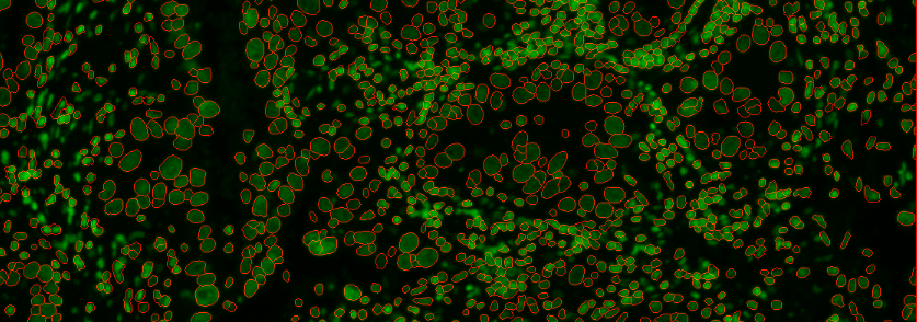
  cellOutlines.ome.tif Cell outlines overlaid with raw image, zoomed in on an arbitrary area. (This example shows the first available cycle (Cycle 6) in the default exemplar-001 data set .)

  Read Parameter Tuning for S3Segmenter for common troubleshooting scenarios.

coreo/

• Check for correct partitioning of TMAs

  

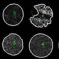
  TMA_MAP.tif exemplar-002

  Read Parameter Tuning for Coreograph for common troubleshooting scenarios.

unmicst/

• Examination of qc/unmicst/ is generally not necessary if qc/s3seg/ outlines are satisfactory

• However, if segmentation results found in qc/s3seg/ are not desirable, UnMICST qc files can provide a clue for what went wrong.

  Read Parameter Tuning for UnMICST for common troubleshooting scenarios.

More details on output files and quality control can be found in Inputs/Outputs.

Table of contents

• Installation